This post was originally written in Turkish and translated into English with AI.
Today I want to touch on something different from company and sector analysis, but far more important: position sizes and their effects across different win-rate scenarios.
In 2016, former LTCM partner Victor Haghani and Rich Dewey ran a deceptively simple experiment. They gave 61 finance-trained participants $25 each and placed a rigged coin in front of them: it landed heads 60% of the time. Participants were free to bet any size they wanted for 30 minutes. In other words, they were handed something no market ever offers — a guaranteed statistical edge. The outcome surprised everyone: roughly a third of the participants lost their entire stake, and two thirds bet on tails (against their own edge) at some point.
The first takeaway is that knowing your edge is not enough. In this piece I will first leave you alone with a trading-focused version of the same problem, then get into what the Kelly criterion is and why most professionals size at half of the “optimum”. Along the way we will follow the line of thinking physicist John L. Kelly started, and look at how it can best be applied in financial markets once human psychology enters the picture.
What is the Kelly Criterion?
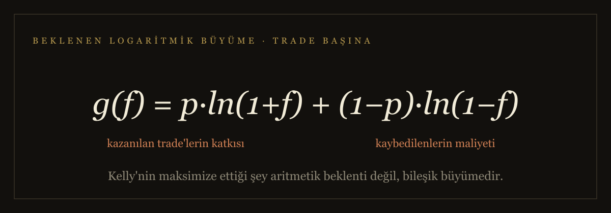
In 1956, John L. Kelly, a physicist at Bell Labs, started from Shannon’s information theory and asked: if I hold a bet with an edge, what fraction of my wealth should I risk so that my long-run compound growth is maximized?
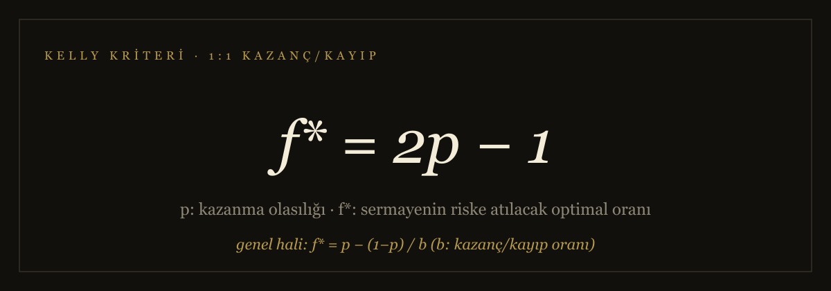
If your win probability is 55%, you should risk 10% of your capital; at 60%, 20% — that is what maximizes your compounding. Plenty of people took the formula into the real world: Ed Thorp carried the same mathematics first to the blackjack tables (Beat the Dealer), then to markets, compounding at roughly 20% a year for two decades at Princeton-Newport with barely a drawdown.
The simulator shows you the optimal position size for a given win rate (10% for a 55% win rate) — that is the Kelly optimum. You are free to raise or lower the size you put on each trade. In this scenario, quarter Kelly corresponds to a 2.5% position and half Kelly to 5%. And if you want to go beyond the optimum, the simulation keeps running with position sizes above 10%.
The Optimum and Ruin Levels
When we express the Kelly criterion (the portfolio percentage to be risked on each hand) as f* and turn it into a chart, an interesting picture emerges. One thing to note: for the sake of visualization we assume the player has unlimited capital — without that assumption, every scenario above f* carries the risk of taking us to ruin.
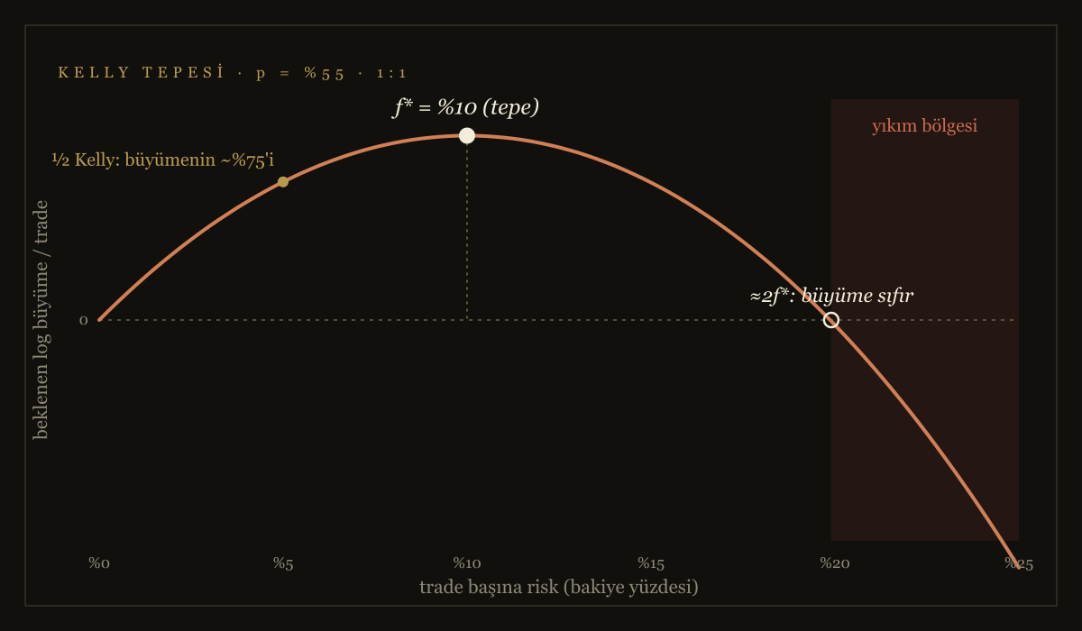
Even at full Kelly, the odds of seeing half your capital at some point are a coin flip. Half Kelly keeps three quarters of the growth while cutting that probability to about 12.5%. The return you give up is, in effect, insurance you are buying.
I touched on the fund-management counterpart of this in the Q2 investor letter. Scaling positions convexly as conviction rises is a strategy many large fund managers rely on. Kelly is the mathematical skeleton of that approach. However high your conviction, beyond 2f* is not courage — arithmetically, it works against the investor.
Finding the Optimum in Loss Psychology
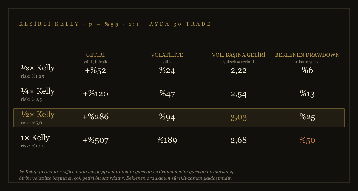
There is one more parameter none of this research can express mathematically: psychology. Even though a full-Kelly size maximizes portfolio returns on paper, the losses along the way — and the poor decisions they trigger — are very likely to work against you in risk-return terms. That is why, for many professional investors, positions sized at ½ or ¼ Kelly are seen as a way to keep compounding while protecting the psyche. The table below shows the data for the different sizing scenarios. Half Kelly is the most efficient size in terms of return per unit of volatility, yet an expected drawdown of around 25% can still strain an investor’s psychology enough to cause long-run losses.
Sources referenced in this piece:
J. L. Kelly Jr., “A New Interpretation of Information Rate” (1956)
V. Haghani & R. Dewey, “Rational Decision-Making Under Uncertainty: Observed Betting Patterns on a Biased Coin” (2016, SSRN)
E. Thorp, “Beat the Dealer” (1962)
Disclaimer
This post has been prepared for informational purposes only and does not constitute investment advice, a recommendation to buy or sell, or an offer relating to any security. The views and analyses expressed here reflect the author’s personal assessments and do not represent the official view of any institution he is affiliated with. Past performance is no guarantee of future results. Every investment carries risk; investors should do their own research and consult a licensed investment advisor where necessary.